3.5 Residuals are Perfectly Balanced at the Mean
What we'd like to do is find the function for a line that perfectly balances the residuals. If the sum of the residuals adds up to 0, then this might just be the best model we can find. Let's do some investigating and see how far this idea can take us.
Residuals Are Balanced at the Mean of a Variable
Let's start with something simpler than a line. You've probably learned about the arithmetic mean, also called the average, before. It's the number you get when you take a set of numbers, add them up, and then divide by the total number of numbers in the set.
For example, there are 333 penguins in the penguins
dataset. Using R, we can calculate the mean (or average) body mass like
this:
# this puts all 333 body masses in a vector Y
Y <- penguins$body_mass_kg

# this adds up all the body masses and divides by 333
sum(Y) / 333 4.20705705705706The mean is so commonly used in data science and statistics that
there is a function in R, called mean(), to calculate it.
You can just put your vector Y directly into it; give it a
try below.
require(coursekata)
# defines our Y
Y <-  penguins$body_mass_kg

# one way of calculating the mean of Y
sum(Y) / 333

# write code to use the function mean()
# creates the vectors Y and X
Y <-  penguins$body_mass_kg
X <-  penguins$flipper_length_m

# one way of calculating the mean of Y
sum(Y) / 333

# write code to use the function mean()
mean(Y)
ex() %>% check_function("mean") %>% check_arg("x") %>% check_equal()We sometimes refer to the mean of a variable as the empty model of that variable. Think of it this way: if DATA = MODEL + ERROR, then there is no predictor variable in the MODEL part of the equation. In the empty model, we replace the MODEL function with just the mean (which is also a function): DATA = MEAN + ERROR.
We could think of residuals from the empty model as just the
residuals from the mean of \(Y\) (body
mass). Here's some code that would calculate those residuals and put
them in a vector called residual_from_mean:
residual_from_mean <- Y - mean(Y)We've put code to calculate the residuals from the mean of
Y into the code window below. Add some code to sum up these
residuals and see what you get.
require(coursekata)
# creates vectors Y and X
Y <-  penguins$body_mass_kg
X <-  penguins$flipper_length_m

# creates vector with residuals from mean of Y
residual_from_mean <- Y - mean(Y)

# write code here to sum up the residuals from mean of Y
# creates vectors Y and X
Y <-  penguins$body_mass_kg
X <-  penguins$flipper_length_m

# creates vector with residuals from mean of Y
residual_from_mean <- Y - mean(Y)

# write code here to sum up the residuals from mean of Y
sum(residual_from_mean)
ex() %>% check_function("sum") %>% check_arg("x") %>% check_equal()
1.23900889548167e-13Notice that the output we got by summing up the residuals from the
mean of Y is almost exactly 0. It's written in
scientific notation, so you may not have immediately noticed this. You
can read it as "-1.239 times 10 to the -13" (the e stands for
exponent.) That means you move the decimal point 15 places to
the left, which gives you the sum of 0.0000000000001239. For all
practical purposes, the sum is equal to 0. (R will not always report the
sum as exactly 0 because of computer hardware limitations but it will be
close enough to 0.)
It turns out this is true for any variable. If you modify the code in
the window above to get the residuals for X
(flipper_length_m) and then sum up those residuals, that
sum will also add up to 0. This turns out to be an interesting and
important fact for statisticians that will actually help us on our quest
for the best model.
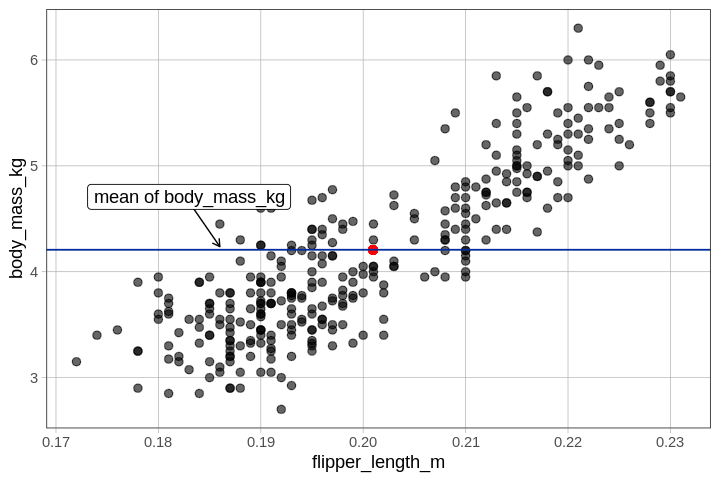
The Point of Means
The mean of Y and the mean of X are crucial
for balancing the residuals. This leads to an interesting fact: Just as
the residuals around the mean of a variable add up to 0, the residuals
around a linear function (the line we are using as a model) will add up
to 0 provided the line passes through the point of
means.
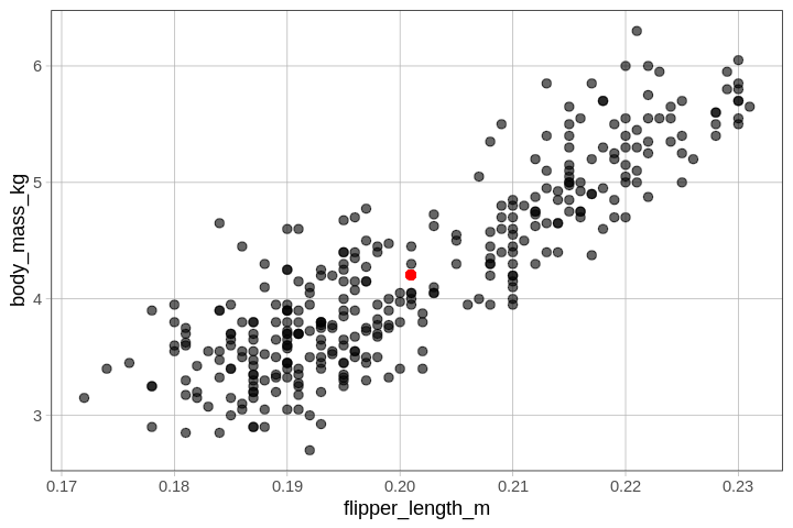
The point of means is simply the point on our scatter plot where the mean of \(Y\) and the mean of \(X\) intersect.
We can plot this special point like this:
gf_point(mean(Y) ~ mean(X))
In the code block below, pipe (%>%) on the point of
means in red onto the basic scatter plot of body mass by flipper
length.
require(coursekata)
# create vectors Y and X
Y <-  penguins$body_mass_kg
X <-  penguins$flipper_length_m

# add the point of means (in red) to this scatter plot
gf_point(body_mass_kg ~ flipper_length_m, data = penguins)
# create vectors Y and X
Y <-  penguins$body_mass_kg
X <-  penguins$flipper_length_m

# add the point of means (in red) to this scatter plot
gf_point(body_mass_kg ~ flipper_length_m, data = penguins) %>%
  gf_point(mean(Y) ~ mean(X), color = "red")
ex() %>% {
  check_function(., "gf_point", index = 1) %>% {
    check_arg(., "object") %>% check_equal()
    check_arg(., "data") %>% check_equal()
  }
  check_function(., "gf_point", index = 2) %>% {
    check_arg(., 1) %>% check_equal()
    check_arg(., 2) %>% check_equal()
  }
}