4.3 Categorical Explanatory Variables

Hypotheses with Categorical Variables

We have learned how to translate hypotheses into word equations and then into scatter plots with a quantitative outcome and a quantitative explanatory variable (Thumb and Height are both quantitative). Now let’s try swapping out the quantitative explanatory variable of Height with a categorical explanatory variable: Gender.

In the code block below, make a scatter plot to explore this hypothesis.

Although this graph might look a little weird at first, it is also a scatter plot! It’s just that Gender is a different kind of variable than Height. There are many values of Height: 59, 60.5, 72, just to name a few (it would be a long list to name them all!). The variable Gender in contrast has only two possible values: “female” or “male”. So the dots are all lined up in one of two places on the horizontal x-axis: above the “female” or above the “male”.

Notice that the variable Thumb still varies quantitatively so the data points are spread out along the vertical y-axis even though they are clustered on the x-axis.

We can look at the graph again in light of the hypothesized relationship we were investigating: Thumb = Gender + other stuff. Does the variable Gender explain some of the variation in Thumb?

If Gender explains some of the variation in Thumb then knowing whether a student is female or male would help us make a better prediction of their thumb length than if we didn’t know what gender they reported. If we know that a student is male, we would predict a longer thumb (maybe 65 mm, the middle of the male distribution) than if the student were female, in which case we might predict something closer to 60 mm. These wouldn’t be very accurate predictions, but they’d be a little bit better than if we didn’t know anything about the gender of the student.

Jitter Plots

Although a scatter plot is a common way to show the relationship between an outcome variable and an explanatory variable, in the case of a categorical explanatory variable (like Gender) we often can’t see all the points because so many of them are on top of other points. One solution to this is to jitter the points around a little so that you can better see the individual points.

We’ll use the function gf_jitter() to create a jitter plot depicting Thumb by Gender. This function works just like gf_point(), except that the points will be randomly jittered both vertically and horizontally. As you can see below, the default jitter plot has an awful lot of jitter!

gf_jitter(Thumb ~ Gender, data = Fingers)

We can use the arguments height and width to adjust the amount of jitter. In this situation, we might want the vertical jitter (height) to be set to 0 so that a person with a thumb length of 60 mm shows up right at 60 on the y-axis. We might also want to reduce the horizontal jitter (width), but not so much that the points overlap too much. Note that these two arguments can be set to values between 0 and 1.

Try running the code below. To submit, reduce the height of the jitter to 0 and the width to 0.1.

If a point is in the Female column, it’s a female’s thumb length. But being more to the left or right within the female column doesn’t mean anything - it’s just random jitter. The jitter is there just so the points do not overlap too much and obscure how many females have that same thumb length.

In the jitter plot, a dense row of points shows that there are a lot of people with that thumb length. For instance, look at all the Female points at 60 mm, shown in purple below. More points means more females with that particular thumb length.

Extra Features for Scatter and Jitter Plots

In both scatter and jitter plots, you can change the size, shape, and transparency of the points by including the arguments size, shape, and alpha, respectively.

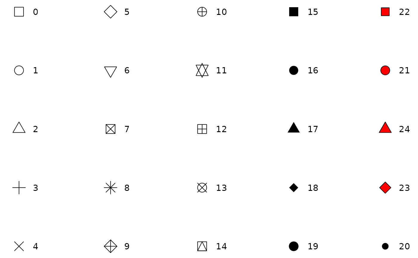
Here are some different shapes you can use. For example, putting in the argument shape = 15 will result in squares rather than circles on a scatter or jitter plot.

Play around with the code below and try changing the size (put in numbers between 0-5 to start), shape (put in whole numbers between 1 and 20), and transparency (put in numbers between 0-1, 0 being more transparent and 1 being more opaque).