1.3 Data Frames
Now for the moment you all have been waiting for: It’s time to work with real data in R! For handling datasets, R has a special object type called a data frame. Data frames look like this:
species gentoo body_mass_kg flipper_length_m bill_length_cm female island
1 Adelie 0 4.200 0.194 4.6 0 Torgersen
2 Gentoo 1 4.375 0.217 4.6 1 Biscoe
3 Adelie 0 3.950 0.185 3.8 0 Biscoe
4 Gentoo 1 5.700 0.218 5.0 0 Biscoe
5 Adelie 0 4.000 0.210 4.4 0 Torgersen
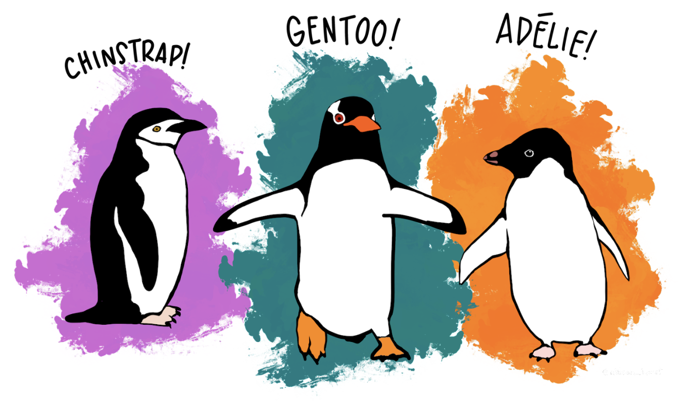
6 Adelie 0 3.000 0.192 3.7 1 DreamThis is the first six rows of a data frame called penguins. The full data frame contains data that were collected at the Palmer Station in Antarctica as part of a study about penguins.
Each row in a data frame represents a single case. In the penguins data frame, the cases (which are sometimes called observations) are penguins. Each row represents one penguin. Depending on the study, the cases (or rows) could be people, states, couples, mice – anything you could take a sample of in order to make a dataset.
  species gentoo body_mass_kg flipper_length_m bill_length_cm female    island
1  Adelie      0        4.200            0.194            4.6      0 Torgersen
2  Gentoo      1        4.375            0.217            4.6      1    Biscoe
3  Adelie      0        3.950            0.185            3.8      0    Biscoe
4  Gentoo      1        5.700            0.218            5.0      0    Biscoe
5  Adelie      0        4.000            0.210            4.4      0 Torgersen
6  Adelie      0        3.000            0.192            3.7      1     Dream
These are the values that go with the first penguin in this data frame.
The columns of the data frame (for example, those that are labeled species or flipper_length_m) represent variables, or the attributes of each case that could vary from row to row.
This dataset is organized in a “tidy” format (a term coined by statistician Hadley Wickham). It’s generally good practice to format our datasets in a tidy way (“keep things tidy”). The key aspects of a tidy dataset are:
 |
 |
 |
|---|---|---|
| 1. Each row is a case (or observation). | 2. Each column is a variable. | 3. Each cell contains a value for the particular case and variable. |
You can read more about the data here: Palmer Penguins data set documentation.
Peeking at a Data Frame
As with any object in R, you can just type the name of the data frame to see the whole thing.
In the code block below, type the name of the data frame penguins and then <Run>.
require(coursekata)
# Try typing penguins to see what is in the data frame.
# Try typing penguins to see what is in the data frame.
penguins
ex() %>% check_output_expr("penguins")Be sure to scroll up and down to see the whole output. Once you do, you might think to yourself, “Wow, that’s a lot to take in!” This is usually the case when working with real data frames, which often include many rows and many columns. Here, we don’t just have data from one penguin—we have a bunch of penguins, each with their own values for different variables.
head() and tail(). It’s often useful to take a quick peek at your data frame without printing out the whole thing. One way to do this is with the head() command.
In the window below, type the command head(penguins) and then press the <Run> button. Look at the output to see what the head() function does.
require(coursekata)
# write code to print the first 6 rows of penguins
# write code to print the first 6 rows of penguins
head(penguins)
ex() %>% check_function("head") %>%
  check_result() %>% check_equal()
species gentoo body_mass_kg flipper_length_m bill_length_cm female island
1 Adelie 0 4.200 0.194 4.6 0 Torgersen
2 Gentoo 1 4.375 0.217 4.6 1 Biscoe
3 Adelie 0 3.950 0.185 3.8 0 Biscoe
4 Gentoo 1 5.700 0.218 5.0 0 Biscoe
5 Adelie 0 4.000 0.210 4.4 0 Torgersen
6 Adelie 0 3.000 0.192 3.7 1 DreamThe head() function (or command) prints out just the first six rows of the data frame. (You can also try the tail() function, which prints the last six rows.)
We can also add an argument to head() to show a different number of rows. What do you think head(penguins, 3) will do? Run the code below to see.
require(coursekata)
# what do you think this code will do? run to find out
# modify it to show 20 rows of the data frame
head(penguins, 3)
# what do you think this code will do? run to find out
# modify it to show 20 rows of the data frame
head(penguins, 20)
ex() %>% check_function("head") %>%
  check_result() %>% check_equal()
From Noticing Variation to Exploring Variation
When you start looking at data, you’ll see that all of a sudden we are in a new kind of math where there isn’t just one number for penguins’ body mass. There are many numbers for body mass! That’s because these penguins vary in body mass. They are different from each other. That’s why we call body_mass_kg a variable – because penguins have different levels of it. In the next pages we will transition from noticing the existence of variation to exploring that variation with a data visualization (a scatter plot).